

Compare your data to mobility laws
Question. Do the movements in my data follow the regularities reported for human mobility, and what are their parameters?
You will get three fitted laws with their parameters and plots (for the distance law also confidence intervals, the effect of the fitted range and a comparison with alternative forms): the truncated power law of jump lengths, the universal visitation law (how often people visit places at each distance), and the lognormal distribution of the number of distinct places a person visits per day.
Prerequisites. Measure individual mobility and Population measures.
Data. Brightkite check-ins (Stanford SNAP, 2008 to 2010): the first 300,000 rows (about 4 MB of the 60 MB file) with fastmob.data.load_brightkite, users with at least 100 check-ins (about 306). For the stay-based laws each check-in is treated as a 30-minute stay (an assumption). The notebook stops if the download fails.
Load and clean
As in the previous notebooks, we drop placeholder and invalid coordinates and users with fewer than 100 check-ins.
import fastmob
import matplotlib.pyplot as plt
import numpy as np
import pandas as pd
from fastmob.data import load_brightkite
from fastmob.measures import fitting

raw = load_brightkite(max_rows=300_000).to_pandas()

raw = raw[~(((raw["lat"] == 0) & (raw["lng"] == 0)) | (raw["lat"].abs() >= 90))]
counts = raw.groupby("uid").size()
checkins = (
    raw[raw["uid"].isin(counts[counts >= 100].index)]
    .sort_values(["uid", "datetime"])
    .reset_index(drop=True)
)
print(len(checkins), "check-ins by", checkins["uid"].nunique(), "users")
Law 1: jump lengths follow a truncated power law
Human jump lengths are heavy-tailed: short moves are common, long ones rare but not negligible, up to a cutoff. fit_values_to_truncated_powerlaw fits \(P(\Delta r) \propto (\Delta r + \Delta r_0)^{-\beta} \exp(-\Delta r / \kappa)\) to a log-spaced histogram of positive jumps and returns the four parameters (c, r0, beta, kappa) plus the histogram it fitted. log_truncated_powerlaw evaluates the fitted curve.
jumps = fastmob.jump_lengths(checkins)
values = np.concatenate(jumps["jump_lengths"].to_list())
values = values[np.isfinite(values) & (values > 0)]
params, x, y = fitting.fit_values_to_truncated_powerlaw(values)
curve = np.exp(fitting.log_truncated_powerlaw(x, *params))

c, r0, beta, kappa = params
print(f"{len(values):,} positive jumps, median {np.median(values):.1f} km")
print(f"beta = {beta:.2f}, r0 = {r0:.2f} km, kappa = {kappa:,.0f} km")
fig, ax = plt.subplots(figsize=(6, 4))
ax.loglog(x, y, "o", ms=4, alpha=0.7, label="Brightkite jump lengths")
ax.loglog(x, curve, "-", lw=2, label="truncated power law")
ax.set_xlabel("jump length (km)")
ax.set_ylabel("density")
ax.legend()
fig.tight_layout()
plt.show()
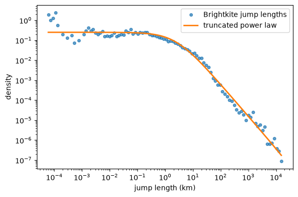
There are 133,372 positive jumps with a median of 7.1 km. The fit gives beta = 1.61 and r0 = 2.4 km: below a few kilometres the density is flat, above it falls as a power law of about -1.6. The cutoff kappa (143,421 km) is far larger than the size of the Earth, so no cutoff is detectable here and the curve is effectively a plain power law up to the longest jumps (about 15,000 km). The curve follows the data over seven orders of magnitude; the points at the shortest lengths (below about 1 m) are noisy.
How sure is the fit? Range, uncertainty and alternatives
The grid-search fit above returns four numbers and nothing about their uncertainty, and it depends on the range of values it sees. fit_distance_distribution fits by maximum likelihood on a stated range, gives a bootstrap confidence interval for each parameter and flags a parameter that the data do not identify. We fit the jump lengths from 1 km upwards (which leaves out the many very short jumps, where check-in positions are not reliable) and up to half the circumference of the Earth, 20,015 km, the longest distance between two places on the planet (the upper limit matters: if it is left at the longest observed jump, that jump becomes the end of the distribution and a cutoff can hide behind it), with 100 bootstrap replicates.
from fastmob.measures.fitting import (
    compare_distance_distributions,
    fit_distance_distribution,
    likelihood_ratio_test,
    select_xmin,
    vuong_test,
)

# half the circumference of the Earth (km): no jump can be longer, so no cutoff hides behind the data
xmax = 20_015.0
fit = fit_distance_distribution(values, "truncated_powerlaw", xmin=1.0, xmax=xmax, n_bootstrap=100)
print(
    f"{fit.n:,} jumps fitted between {fit.xmin:g} and {fit.xmax:,.0f} km;",
    f"{fit.n_excluded:,} left out; KS distance {fit.ks_statistic:.3f};",
    "at the edge of the search range:",
    fit.at_bound or "none",
)
fit.summary().to_pandas().round(3)
111,012 jumps fitted between 1 and 20,015 km; 22,360 left out; KS distance 0.045; at the edge of the search range: ('kappa',)
| parameter | estimate | std_error | ci_low | ci_high | at_bound | |
|---|---|---|---|---|---|---|
| 0 | r0 | 4.990000e+00 | 0.072 | 4.873 | 5.140 | False |
| 1 | beta | 1.766000e+00 | 0.005 | 1.758 | 1.778 | False |
| 2 | kappa | 2.001500e+07 | NaN | NaN | NaN | True |
The fit uses 111,012 jumps between 1 km and 20,015 km; the other 22,360 positive jumps are shorter than 1 km. The exponent is beta = 1.77 (95% interval 1.76 to 1.78) and the shift r0 = 5.0 km (4.9 to 5.1). The cutoff kappa ended on the edge of its search range, 20 million km, 1,000 times the longest possible jump: the data do not identify a cutoff, so its interval is meaningless and the "truncated" power law fitted here is in effect a shifted power law. This is the same finding as above (kappa = 143,421 km), now stated by the fit itself in at_bound. The KS distance is 0.045: the largest gap between the empirical and the fitted cumulative distribution is 4.5 percentage points. The very narrow interval of beta reflects 111,000 jumps in a sample of 306 people who contribute very unequally; it describes the fitting error, not how well it would transfer to other people.
The grid-search fit above gave beta = 1.61 and r0 = 2.4 km. The two differ because the estimators and the ranges differ (the grid search uses a log histogram of all the positive jumps, this fit starts at 1 km); report the maximum-likelihood values, with the range and the interval.
owner = np.repeat(jumps["uid"].to_numpy(), jumps["jump_lengths"].map(len).to_numpy())
everything = np.concatenate(jumps["jump_lengths"].to_list())
by_user = fit_distance_distribution(
    everything, "truncated_powerlaw", xmin=1.0, xmax=xmax, n_bootstrap=100, groups=owner
)
pd.DataFrame(
    {
        "jumps resampled": [
            fit.std_errors["beta"],
            fit.ci_low["beta"],
            fit.ci_high["beta"],
        ],
        "users resampled": [
            by_user.std_errors["beta"],
            by_user.ci_low["beta"],
            by_user.ci_high["beta"],
        ],
    },
    index=["std error of beta", "95% low", "95% high"],
).round(3)
| jumps resampled | users resampled | |
|---|---|---|
| std error of beta | 0.005 | 0.036 |
| 95% low | 1.758 | 1.706 |
| 95% high | 1.778 | 1.844 |
Resampling users instead of jumps changes the answer a lot: the standard error of beta goes from 0.005 to 0.036 and the 95% interval from 1.76 to 1.78 to 1.71 to 1.84. The 111,000 jumps come from 306 people whose habits differ, so the jumps are far from independent. When the values come from a limited number of people, pass groups= and report that interval.
Is the truncated power law better than simpler or different forms? compare_distance_distributions fits the five families on the same range and ranks them by AIC (lower is better; an Akaike weight is the relative support among the families listed).
| family | n_parameters | log_likelihood | aic | bic | delta_aic | akaike_weight | ks_statistic | gof_p_value | at_bound | degenerate | |
|---|---|---|---|---|---|---|---|---|---|---|---|
| 0 | shifted_powerlaw | 2 | -532856.190 | 1065716.380 | 1065735.615 | 0.000 | 0.784 | 0.045 | None | False | |
| 1 | truncated_powerlaw | 3 | -532856.479 | 1065718.957 | 1065747.810 | 2.577 | 0.216 | 0.045 | None | kappa | False |
| 2 | lognormal | 2 | -536286.170 | 1072576.339 | 1072595.574 | 6859.959 | 0.000 | 0.071 | None | False | |
| 3 | powerlaw | 1 | -545229.370 | 1090460.740 | 1090470.358 | 24744.360 | 0.000 | 0.137 | None | False | |
| 4 | exponential | 1 | -724434.050 | 1448870.100 | 1448879.717 | 383153.720 | 0.000 | 0.614 | None | False |
The AIC ranks the shifted power law (two parameters, r0 and beta) first. The truncated power law adds the cutoff, but its kappa is on the upper edge of its range, which is the legitimate limit of no cutoff (it is not degenerate), so it fits the same curve with one more parameter: it is 2.6 AIC units behind and the Akaike weights are 0.78 and 0.22, which says that the data cannot tell them apart and nothing more. The plain power law is 24,744 units behind the shifted one, so the shift r0 matters (it flattens the density below a few kilometres); the log-normal is 6,860 behind and the exponential far further. With 111,000 jumps even small differences are decisive, so read this as ordering, and check the fit against the data as well. These gaps come from 111,000 jumps of 306 people, who are not independent, so they overstate the evidence in the same way the first intervals did: read the ordering, not the size of the gaps.
Does the data need a cutoff, and does a different family fit better?
The ranking above is a comparison of numbers. Two tests answer the questions behind it. likelihood_ratio_test asks whether the truncated power law is better than the shifted one it extends, and vuong_test whether two families that are not nested (here the shifted power law and the log-normal) fit differently. Because a cutoff that the data do not show leaves kappa on the edge of its range, fit.profile("kappa") gives the profile-likelihood interval, which says what the data do show about the cutoff, and bounds= lets us check that the answer does not depend on the search range.
shifted = fit_distance_distribution(values, "shifted_powerlaw", xmin=1.0, xmax=xmax, n_bootstrap=0)
truncated = fit_distance_distribution(values, "truncated_powerlaw", xmin=1.0, xmax=xmax, n_bootstrap=0)
lognormal = fit_distance_distribution(values, "lognormal", xmin=1.0, xmax=xmax, n_bootstrap=0)

cutoff_test = likelihood_ratio_test(shifted, truncated, n_bootstrap=100)
print(f"cutoff: statistic {cutoff_test.statistic:.1f}, bootstrap p = {cutoff_test.p_value:.3f}; {cutoff_test.note}")
print(truncated.profile("kappa"))

wider = fit_distance_distribution(
    values, "truncated_powerlaw", xmin=1.0, xmax=xmax, n_bootstrap=0, bounds={"kappa": (1.0, 1e7)}
)
print(f"with kappa searched up to 10 million km: kappa = {wider.parameters['kappa']:,.0f} km, at the edge: {wider.at_bound}")

family_test = vuong_test(shifted, lognormal)
print(f"shifted power law against log-normal: z = {family_test.statistic:.1f}; {family_test.note}")
cutoff: statistic 0.0, bootstrap p = 1.000; the data do not need the extra terms of truncated_powerlaw; shifted_powerlaw is enough


kappa >= 2.619e+06 (95%; no upper limit), estimate 2.001e+07


with kappa searched up to 10 million km: kappa = 10,000,000 km, at the edge: ('kappa',)
shifted power law against log-normal: z = 68.1; shifted_powerlaw is supported
The likelihood-ratio statistic is 0.0, so the truncated power law fits no better than the shifted one (bootstrap p = 1): the data do not need a cutoff. The profile of kappa says the same in quantitative form: at 95% the cutoff is at least 2.6 million km and has no upper limit, while the longest jump is about 17,000 km, so there is no cutoff anywhere in the range of possible jumps. Searching kappa up to 10 million km only moves the fitted value to the new edge, so the missing cutoff does not depend on the search range. Against the log-normal, the Vuong statistic is 68.1 in favour of the shifted power law. These tests treat the 111,000 jumps as independent, so read them as direction, not as the size of the evidence.
The lower limit of 1 km was a choice. select_xmin fits a grid of lower limits and picks the one with the smallest KS distance (Clauset et al., 2009); the table shows how the exponent moves along the grid.
selection = select_xmin(values, "shifted_powerlaw", candidates=np.geomspace(0.1, 100, 10), xmax=xmax)
selection.to_pandas().round(3)
| xmin | n | ks_statistic | log_likelihood | r0 | beta | at_bound | selected | |
|---|---|---|---|---|---|---|---|---|
| 0 | 0.100 | 130215 | 0.038 | -632915.031 | 4.052 | 1.724 | True | |
| 1 | 0.215 | 126559 | 0.038 | -615099.472 | 4.318 | 1.737 | False | |
| 2 | 0.464 | 120362 | 0.041 | -582421.471 | 4.702 | 1.754 | False | |
| 3 | 1.000 | 111012 | 0.045 | -532856.190 | 4.990 | 1.766 | False | |
| 4 | 2.154 | 97013 | 0.052 | -460432.331 | 4.937 | 1.764 | False | |
| 5 | 4.642 | 78319 | 0.060 | -366905.883 | 3.871 | 1.737 | False | |
| 6 | 10.000 | 57242 | 0.064 | -264497.785 | 0.100 | 1.683 | r0 | False |
| 7 | 21.544 | 33063 | 0.103 | -156163.161 | 0.215 | 1.670 | r0 | False |
| 8 | 46.416 | 16343 | 0.066 | -82112.639 | 0.464 | 1.465 | r0 | False |
| 9 | 100.000 | 10185 | 0.074 | -52587.143 | 3.286 | 1.362 | False |
The KS distance is smallest at the lowest candidates (0.1 and 0.2 km) and grows with xmin, while the exponent moves from 1.72 to 1.77 and back to 1.68 and 1.36 at 10 and 100 km. So the data do not ask for a lower limit: the shifted power law describes the short jumps as well as the long ones. The choice of 1 km above comes from the doubtful accuracy of check-in positions, not from the data, and it should be reported as such with the range table below.
The estimates depend on the range. We repeat the fit with three lower limits:
rows = []
for xmin in (0.1, 1.0, 10.0):
    f = fit_distance_distribution(
        values, "truncated_powerlaw", xmin=xmin, xmax=xmax, n_bootstrap=50
    )
    rows.append(
        {
            "xmin (km)": xmin,
            "jumps": f.n,
            "beta": f.parameters["beta"],
            "beta 95% interval": f"{f.ci_low['beta']:.2f} to {f.ci_high['beta']:.2f}",
            "kappa (km)": f.parameters["kappa"],
            "at the edge": ", ".join(f.at_bound),
        }
    )
pd.DataFrame(rows).round(2)
| xmin (km) | jumps | beta | beta 95% interval | kappa (km) | at the edge | |
|---|---|---|---|---|---|---|
| 0 | 0.1 | 130215 | 1.72 | 1.72 to 1.73 | 20015000.0 | kappa |
| 1 | 1.0 | 111012 | 1.77 | 1.76 to 1.78 | 20015000.0 | kappa |
| 2 | 10.0 | 57242 | 1.68 | 1.68 to 1.69 | 20015000.0 | r0, kappa |
The exponent depends on the range: beta is 1.72, 1.77 and 1.68 for lower limits of 0.1, 1 and 10 km. The intervals in this table resample jumps, which cell 12 showed to be far too narrow (the interval that resamples people at 1 km is 1.71 to 1.84), so they do not say whether the differences of 0.05 to 0.09 are real; they are of the size of the uncertainty about people. At every lower limit kappa is at its bound, and above 10 km r0 also reaches its lower bound, which means the data there are a plain power law. When you compare with a published exponent, compare on the same range and say which range you used.
Radius of gyration
The same tools apply to the radius of gyration, one value per person. With 306 people the intervals are wide, and a family with many parameters cannot be told apart from a simpler one.
radii = fastmob.radius_of_gyration(checkins)["radius_of_gyration"]
radius_fit = fit_distance_distribution(
    radii, "truncated_powerlaw", xmin=1.0, xmax=xmax, n_bootstrap=100
)
print(
    f"{radius_fit.n} people with a radius of at least 1 km;",
    "at the edge of the search range:",
    radius_fit.at_bound or "none",
)
radius_fit.summary().to_pandas().round(2)
| parameter | estimate | std_error | ci_low | ci_high | at_bound | |
|---|---|---|---|---|---|---|
| 0 | r0 | 0.01 | NaN | NaN | NaN | True |
| 1 | beta | 0.18 | 0.08 | 0.01 | 0.30 | False |
| 2 | kappa | 1230.27 | 163.09 | 923.93 | 1562.76 | False |
compare_distance_distributions(radii, xmin=1.0, xmax=xmax).to_pandas()[
    ["family", "aic", "delta_aic", "akaike_weight", "at_bound"]
].round(2)
| family | aic | delta_aic | akaike_weight | at_bound | |
|---|---|---|---|---|---|
| 0 | truncated_powerlaw | 2861.04 | 0.00 | 0.87 | r0 |
| 1 | exponential | 2864.92 | 3.88 | 0.13 | |
| 2 | lognormal | 2921.20 | 60.16 | 0.00 | |
| 3 | powerlaw | 3163.23 | 302.19 | 0.00 | |
| 4 | shifted_powerlaw | 2859.86 | -1.18 | NaN | beta |
Among the 304 people with a radius of at least 1 km, the table needs care. The shifted power law has beta on the edge of its range (6, the largest allowed): an exponential-like curve forced into a power-law form, so it is listed last as degenerate, with no weight, and its higher likelihood (a delta_aic of -1.2) is what the degeneracy buys. The truncated power law has r0 on its lower edge, which is a legitimate limit (a power law with an exponential cutoff), so it is ranked: first, with a weight of 0.87, and the exponential is 3.9 AIC units behind (0.13). The log-normal is 60 units behind and the plain power law 302. The truncated fit is r^-0.18 exp(-r / 1,230 km): with an exponent that small it is close to an exponential, whose scale is about 1,000 km, and the interval of beta (0.01 to 0.30) reaches the lower edge of its range. So the radii decay like an exponential with a scale of about 1,000 km, and a power-law exponent is not what they show: do not report one. The jump lengths are the opposite case, with a power-law exponent and no cutoff.
kappa >= 1024 (95%; no upper limit), estimate 1230; beta, r0 at a bound along the profile


beta >= 0.05779 (95%; no upper limit), estimate 0.1835; kappa, r0 at a bound along the profile
The bootstrap interval of kappa above (924 to 1,563 km) looks as if the cutoff were identified, but the profile likelihood reports that at 95% kappa is at least 1,024 km with no upper limit, and that beta and r0 reach the edge of their range along the profile. The open end comes from that degenerate shape, the steep shifted power law with beta at 6, which imitates an exponential, and not from a missing cutoff. All the descriptions that are not degenerate agree: an exponential decay with a scale of about 1,000 km (the exponential fit gives 1,000 km, the truncated fit 1,230 km). What the 304 radii cannot decide is whether this is an exponential or a steep power law with a large shift; what they do show is that there is no power-law exponent to report.
Law 2: the universal visitation law
The visitation law (Schläpfer et al., Nature 2021) describes the density \(\rho\) of visitors (visitors per km²) of places that are visited with frequency \(f\) from distance \(r\): it falls as a power of the product \(rf\), \(\rho = \mu (rf)^{-\eta}\). fit_visitation_law takes stays (here the 30-minute check-in stays on an H3 grid of resolution 8), computes the distance \(r\) of each place from the person's home and its distinct-day visit frequency \(f\), bins the values and fits \(\eta\) and \(\mu\) on a log-log scale. The result is a VisitationLawFit with the per-user-place data, the aggregate spectrum that was fitted, and the parameters.
stays = fastmob.Staypoints(
    pd.DataFrame(
        {
            "uid": checkins["uid"],
            "lat": checkins["lat"],
            "lng": checkins["lng"],
            "started_at": checkins["datetime"],
            "finished_at": checkins["datetime"] + pd.Timedelta(minutes=30),
        }
    )
)
places, stays_at = stays.generate_global_locations(h3_resolution=8)
visitation = fitting.fit_visitation_law(stays_at, locations=places)

print(
    f"eta = {visitation.eta:.2f}, mu = {visitation.mu:.2f}, R2 = {visitation.r2:.2f}; {len(visitation.data)} user-place pairs, {len(visitation.spectrum)} spectrum points"
)
visitation.spectrum.head()
| rf | rho | |
|---|---|---|
| 0 | 0.637364 | 0.363783 |
| 1 | 1.035673 | 0.337959 |
| 2 | 1.682898 | 0.177953 |
| 3 | 2.734594 | 0.117504 |
| 4 | 4.443529 | 0.065546 |
spectrum = visitation.spectrum
fig, ax = plt.subplots(figsize=(6, 4))
ax.loglog(spectrum["rf"], spectrum["rho"], "o", label="data")
ax.loglog(
    spectrum["rf"],
    visitation.mu * spectrum["rf"] ** -visitation.eta,
    "-",
    label=f"fit, eta = {visitation.eta:.2f}",
)
ax.set_xlabel("rf (km x visits per day)")
ax.set_ylabel("rho")
ax.legend()
fig.tight_layout()
plt.show()
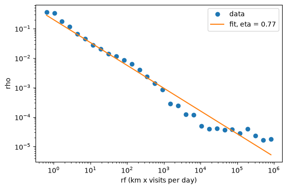
The fitted exponent is eta = 0.77 with R² = 0.97 on 30 spectrum points. The line follows the data over the middle of the range; for rf above about 10⁵ (km per visit per day) the data flatten and lie above the line, so the power law describes the bulk and not the far tail. The exponent is not directly comparable with the published value: that is estimated from mobile-phone data, and check-ins from a social network with an assumed 30-minute stay, in a coarser region of the rf range, can give a different exponent. Compare with the literature for your own kind of data before interpreting eta.
Law 3: distinct places per day are lognormal
fit_daily_location_lognormal counts, for each person and day, the number of distinct places visited, and fits a lognormal distribution to those counts. It returns the values (1, 2, 3, ... places), their observed probability, and the fitted \(\mu\) and \(\sigma\) of the lognormal.
n_places, observed, mu, sigma = fitting.fit_daily_location_lognormal(
    stays_at, locations=places
)

print(
    f"mu = {mu:.2f}, sigma = {sigma:.2f}; share of person-days with 1 place: {observed[0]:.0%}, with 2 places: {observed[1]:.0%}"
)
k = np.array(n_places)
pdf = np.exp(-((np.log(k) - mu) ** 2) / (2 * sigma**2)) / (
    k * sigma * np.sqrt(2 * np.pi)
)
fig, ax = plt.subplots(figsize=(6, 4))
ax.semilogy(k, observed, "o", label="data")
ax.semilogy(k, pdf / pdf.sum() * sum(observed), "-", label="lognormal fit")
ax.set_xlabel("distinct places in a day")
ax.set_ylabel("probability")
ax.legend()
fig.tight_layout()
plt.show()
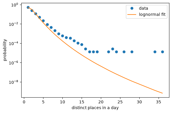
Fitted mu = 0.44 and sigma = 0.54. 55% of the person-days have a single place and 25% have two. The lognormal follows the first few points but falls well below the data from about 8 places a day on: the observed tail is heavier, with a few person-days of 20 to 35 places. For these data a heavier-tailed distribution would fit better.
Interpretation and limits
- A fitted exponent is only meaningful with an uncertainty and a stated range. The distance law has both (
fit_distance_distribution); the visitation-law and log-normal fits above still report point estimates, so do not over-read differences in the second decimal. - Check-in data over-represent short, social, urban movement and skip travel that is not checked in. Compare with literature values only for similar data types (mobile-phone, GPS or check-in data give different parameters).
- The visitation-law and lognormal fits depend on the assumed 30-minute stay and the grid resolution (H3 level 8).
- For the distance law the alternatives are compared by AIC; the visitation law and the daily-places law are judged by eye and by \(R^2\) of the spectrum, without a goodness-of-fit test. With this many observations a test would reject any simple form; see How the fits work.
Next steps
- How the estimators work and what to report: How the fits work.
- Check flows and a distance exponent against a reference table: Validate against census flows.
- The whole cycle on GPS tracks, with a gravity distance decay and a held-out comparison: Validate mobility with GeoLife.
- Compare the fitted law with a model, and quantify the difference: Fit and compare distributions.
- Generate trajectories that follow these laws: Generate mobility with models.
Related API
fit_values_to_truncated_powerlaw ·
log_truncated_powerlaw ·
fit_distance_distribution ·
compare_distance_distributions ·
DistributionFit ·
fit_visitation_law ·
VisitationLawFit ·
fit_daily_location_lognormal