

Chart your results
Question. How do I turn the tables that Fastkit-Mobility returns into charts that I can read, compare and share?
You will get about twenty charts: distributions of jump lengths and radii of gyration, bars, boxes, scatters and a heatmap from per-person tables, and the chart for each kind of result that the library produces (activities, mobility profiles, motifs and the fitted mobility laws).
Prerequisites. Measure individual mobility and Visit-based measures show where the tables come from. The charts need the optional fastmob-vis package (pip install "fastmob[vis]").
Data. Two public samples: 300,000 Brightkite check-ins (a location-sharing service, 2008 to 2010) and six users of the GeoLife GPS data set, which we reduce to visits to places. Both are downloaded the first time.
How charts are made
Every chart is made in one call from a table and the names of its columns. The call returns a chart object (a description of the chart, not a picture). In a live notebook, a chart left as the last expression of a cell is drawn interactively, with tooltips. This page shows the same charts as static pictures.
Two kinds of function make charts:
- Generic charts (
ecdf,bar,scatter,heatmap,boxplot,map) are infastmob.vis. They take any pandas or Polars table and the names of the columns to draw. - Result-specific charts (
plot_jump_lengths_ecdf,plot_visit_purpose_distribution,plot_mobility_profilesand so on) are infastmob_vis. Each expects the shape of one particular result and sets the labels, units and colours for it.
We start with check-ins.
import fastmob
import numpy as np
import pandas as pd
from fastmob import vis
from fastmob.data import load_brightkite

raw = load_brightkite(max_rows=300_000).to_pandas()
raw = raw[~(((raw["lat"] == 0) & (raw["lng"] == 0)) | (raw["lat"].abs() >= 90))]
counts = raw.groupby("uid").size()
checkins = (
    raw[raw["uid"].isin(counts[counts >= 100].index)]
    .sort_values(["uid", "datetime"])
    .reset_index(drop=True)
)

users = np.sort(checkins["uid"].unique())
in_a = checkins["uid"].isin(users[::2])
sample_a, sample_b = checkins[in_a], checkins[~in_a]
print(
    f"sample A: {sample_a['uid'].nunique()} users, {len(sample_a):,} check-ins;",
    f"sample B: {sample_b['uid'].nunique()} users, {len(sample_b):,} check-ins",
)
We removed check-ins at exactly latitude 0 and longitude 0 (a placeholder for "unknown") and impossible latitudes, kept users with at least 100 check-ins, and split the users into two samples: sample A is every second user in sorted order and sample B is the rest. The split is arbitrary. It gives us two groups to compare.
A distribution from one result
ecdf draws the empirical cumulative distribution function: for each value on the horizontal axis, the share of observations that are at most that value. The column can hold one number per row or, as jump_lengths returns, one list of numbers per person; the lists are flattened. The curve stops at the 98th percentile (cdf_cutoff) so that a few very long jumps do not stretch the axis.
jumps_a = fastmob.jump_lengths(sample_a)
jumps_b = fastmob.jump_lengths(sample_b)
flat = lambda frame: np.concatenate(frame["jump_lengths"].to_list())

vis.ecdf(
    jumps_a,
    value_col="jump_lengths",
    x_label="jump length",
    x_unit="km",
    title="Jump lengths",
)
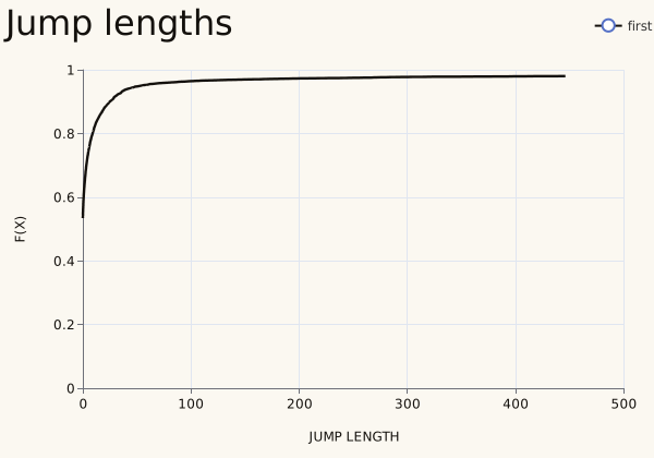
Jump lengths are great-circle distances in kilometres. The curve starts at about 0.53: a little over half of the jumps have length 0, because people check in twice in a row at the same place. It then rises quickly, and the curve stops at 0.98, the cut-off, at about 450 km. The horizontal axis is stretched by a few very long jumps, so the bulk of the distribution is squeezed against the left edge.
Two results on the same axes
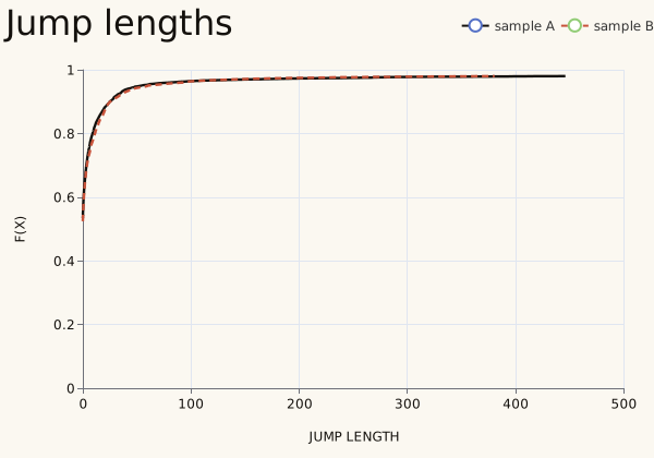
Pass the second result as second and name the two series with labels. This is the standard way to compare an observed result with a simulated one, or two groups of people.
vis.ecdf(
    jumps_a,
    value_col="jump_lengths",
    second=jumps_b,
    labels=("sample A", "sample B"),
    x_label="jump length",
    x_unit="km",
    title="Jump lengths",
)
a, b = flat(jumps_a), flat(jumps_b)
rows = [
    "share of zero-length jumps",
    "median (km)",
    "90th percentile (km)",
    "98th percentile (km)",
]
pd.DataFrame(
    {
        "sample A": [np.mean(a == 0), *np.quantile(a, [0.5, 0.9, 0.98])],
        "sample B": [np.mean(b == 0), *np.quantile(b, [0.5, 0.9, 0.98])],
    },
    index=rows,
).round(2)
| sample A | sample B | |
|---|---|---|
| share of zero-length jumps | 0.53 | 0.52 |
| median (km) | 0.00 | 0.00 |
| 90th percentile (km) | 24.94 | 25.30 |
| 98th percentile (km) | 446.23 | 380.74 |
The two samples are almost the same here. In both, about half of the jumps have length 0, the median is 0 km and nine in ten jumps are shorter than 25 km. They differ only in the far tail: the 98th percentile is 446 km in sample A and 381 km in sample B. Because of the long tail, quantiles such as these tell you more than the shape of the curve.
Bars, boxes, points and a heatmap from a table
The other generic charts take a table with one row per bar, box or point, plus the names of the columns to draw. We build a per-person table of the radius of gyration and the number of distinct places, each with its sample.
people = fastmob.radius_of_gyration(checkins).merge(
    fastmob.number_of_locations(checkins), on="uid"
)
people["sample"] = np.where(people["uid"].isin(users[::2]), "A", "B")
people.sort_values("radius_of_gyration", ascending=False).head(5).round(0)
| uid | radius_of_gyration | number_of_locations | sample | |
|---|---|---|---|---|
| 206 | 427 | 13435.0 | 82 | A |
| 280 | 638 | 5944.0 | 224 | A |
| 212 | 44 | 5588.0 | 76 | A |
| 194 | 4 | 5381.0 | 216 | A |
| 281 | 639 | 5365.0 | 141 | B |
bar draws one bar per category; here the eight people who range the furthest.
vis.bar(
    people.nlargest(8, "radius_of_gyration"),
    category_col="uid",
    value_col="radius_of_gyration",
    title="Widest-ranging people",
)
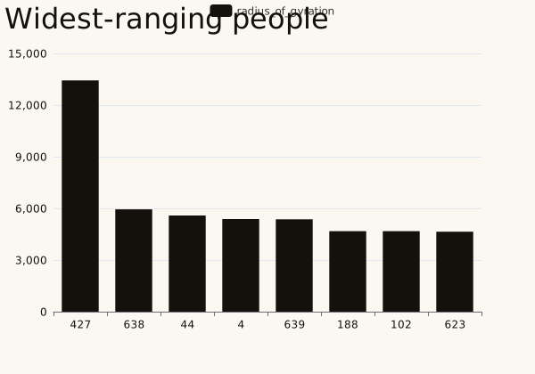
The widest-ranging person (id 427) has a radius of gyration of about 13,400 km, more than twice the next (5,900 km): someone who checked in on several continents. A bar chart ranks people well, but one outlier flattens the rest. The generic charts have no unit on their axes, so say the unit in the text: here, kilometres.
boxplot summarises a column for each category: the box spans the quartiles, the line inside it is the median and the whiskers reach the minimum and maximum. Unlike a bar it shows the spread within each sample.
vis.boxplot(
    people,
    category_col="sample",
    value_col="radius_of_gyration",
    title="Radius of gyration",
)
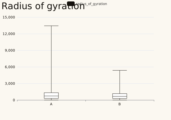
Both samples have a median radius near 700 km (729 km in sample A, 664 km in sample B) and their boxes overlap almost completely, so there is no sign of a difference. The whiskers reach 13,400 km in sample A and 5,400 km in sample B: the longest whisker in A is the outlier above.
scatter draws one point per row; series_col colours the points by group.
vis.scatter(
    people,
    x_col="radius_of_gyration",
    y_col="number_of_locations",
    series_col="sample",
    title="Range and places",
)
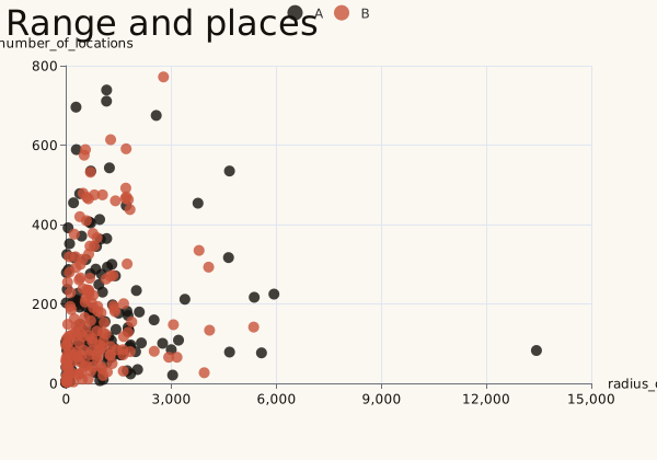
Each point is one person. People who range far do not necessarily visit many places: the rank correlation between the radius and the number of places is only 0.23. The two samples overlap everywhere.
heatmap takes a long table of x, y and a value, one row per cell. We count check-ins by weekday and hour of the day.
when = checkins["datetime"].dt
grid = (
    checkins.assign(
        weekday=when.day_of_week.map(
            dict(enumerate(["Mon", "Tue", "Wed", "Thu", "Fri", "Sat", "Sun"]))
        ),
        hour=when.hour.astype(str).str.zfill(2),
        day=when.day_of_week,
    )
    .groupby(["hour", "day", "weekday"])
    .size()
    .rename("check-ins")
    .reset_index()
)

vis.heatmap(
    grid,
    x_col="hour",
    y_col="weekday",
    value_col="check-ins",
    title="Check-ins by hour",
)
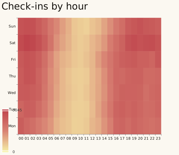
Each cell counts the check-ins of one hour on one weekday, in UTC. Most users are in the United States, so the dark cells from 23:00 to 04:00 UTC are the afternoon and evening there, and the pale band around 10:00 UTC is the night (3 to 6 am). The busiest hour (01:00) has 5.5 times as many check-ins as the quietest (10:00), and Saturday is the busiest day. Cells with no check-ins are left empty.
Charts for one kind of result
The rest of the charts are made for the results of particular functions. They take the result as it comes, with the labels and units already set. Start with the same two samples of check-ins; each of these functions takes two arrays and draws their ECDFs together.
from fastmob_vis import (
    plot_jump_lengths_ecdf,
    plot_radius_of_gyration_ecdf,
    plot_visits_frequency_ecdf,
)

labels = ("sample A", "sample B")

plot_jump_lengths_ecdf(flat(jumps_a), flat(jumps_b), labels=labels)
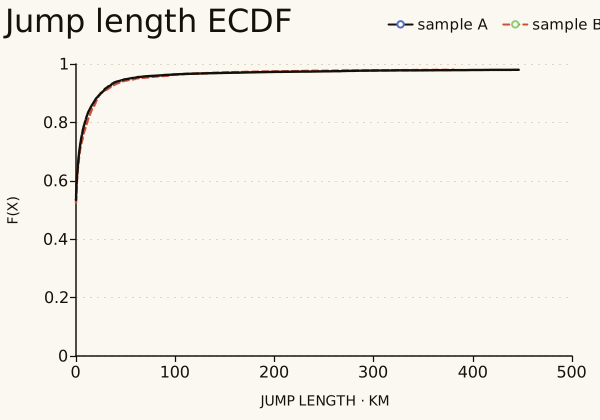
plot_jump_lengths_ecdf draws the same curves from two arrays, with the title, the axis label ("jump length", km) and the legend already set. It is the quickest way to compare a result with a simulation. The result-specific functions below all work like this and return a figure that draws itself.
by_sample = people.groupby("sample")
plot_radius_of_gyration_ecdf(
    by_sample.get_group("A")["radius_of_gyration"],
    by_sample.get_group("B")["radius_of_gyration"],
    labels=labels,
)
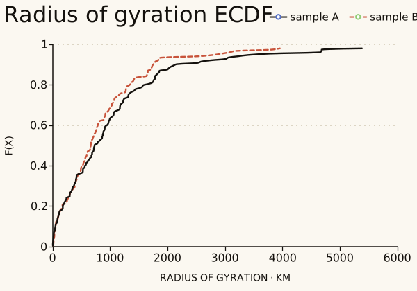
Sample B's curve lies above sample A's over most of the range, so its people tend to range less: the median radius of gyration is 664 km in B and 729 km in A, and A has the longer tail.
visits_per_person = fastmob.number_of_visits(checkins)
visits_per_person["sample"] = np.where(
    visits_per_person["uid"].isin(users[::2]), "A", "B"
)
by_sample = visits_per_person.groupby("sample")
plot_visits_frequency_ecdf(
    by_sample.get_group("A")["number_of_visits"],
    by_sample.get_group("B")["number_of_visits"],
    labels=labels,
)
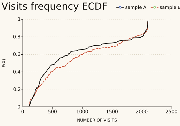
This ECDF is of the number of check-ins per person. Sample A's curve is above sample B's, so its people check in less often: the median is 549 check-ins in A and 775 in B. Both curves end at 2,100 check-ins, the largest number of check-ins of one person in these data.
Mobility laws and their fits
The fitting functions in fastmob.measures.fitting return the parameters of a fitted law together with the points that were fitted. plot_truncated_powerlaw_fits, plot_distance_frequency_law and plot_lognormal_fits draw the points and the fitted curve on the axes that the law is usually shown on, and, with show_reference=True, a reference curve from the literature. They only draw: Compare to mobility laws explains the fits. Each function takes one or more tuples, so several data sets go on one chart.
from fastmob.measures import fitting
from fastmob_vis import (
    plot_distance_frequency_law,
    plot_lognormal_fits,
    plot_truncated_powerlaw_fits,
)

jump_values = np.concatenate([flat(jumps_a), flat(jumps_b)])
jump_values = jump_values[np.isfinite(jump_values) & (jump_values > 0)]
params, x, y = fitting.fit_values_to_truncated_powerlaw(jump_values)

stays = fastmob.Staypoints(
    pd.DataFrame(
        {
            "uid": checkins["uid"],
            "lat": checkins["lat"],
            "lng": checkins["lng"],
            "started_at": checkins["datetime"],
            "finished_at": checkins["datetime"] + pd.Timedelta(minutes=30),
        }
    )
)
places, stays_at = stays.generate_global_locations(h3_resolution=8)
visitation = fitting.fit_visitation_law(stays_at, locations=places)
n_places, observed, mu, sigma = fitting.fit_daily_location_lognormal(
    stays_at, locations=places
)

print(f"beta = {params[2]:.2f}, r0 = {params[1]:.2f} km, kappa = {params[3]:,.0f} km")
print(f"visitation law: eta = {visitation.eta:.2f}, mu = {visitation.mu:.2f}")
print(f"daily places: mu = {mu:.2f}, sigma = {sigma:.2f}")
plot_truncated_powerlaw_fits((params, x, y, "Brightkite"))
beta = 1.61, r0 = 2.40 km, kappa = 143,421 km
visitation law: eta = 0.77, mu = 0.20
daily places: mu = 0.44, sigma = 0.54
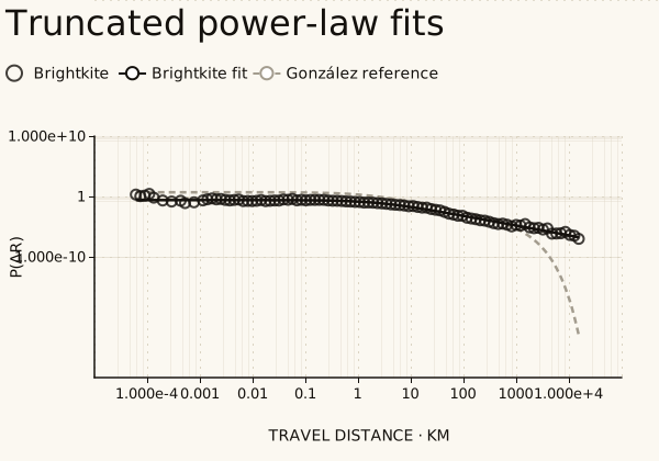
The points are the distribution of jump lengths and the line is the fitted truncated power law (beta = 1.61, r0 = 2.40 km, kappa = 143,421 km), on logarithmic axes. The dashed line is the reference of González et al. (2008), with a cut-off of 400 km: it falls steeply beyond a few thousand kilometres, where the fit, whose cut-off is far beyond any distance on Earth, does not.
spectrum = visitation.spectrum
plot_distance_frequency_law(
    (spectrum["rf"], spectrum["rho"], visitation.eta, visitation.mu, "Brightkite")
)
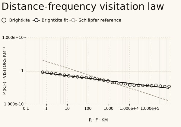
The points are the visitation spectrum, the density of visitors against the product of distance and visit frequency, and the line is the fit with slope -eta = -0.77. The dashed line is the reference slope of -2 of Schläpfer et al. (2021). The slope fitted here is much shallower, so with these data the law does not hold with its published exponent. Compare to mobility laws runs the same fit.
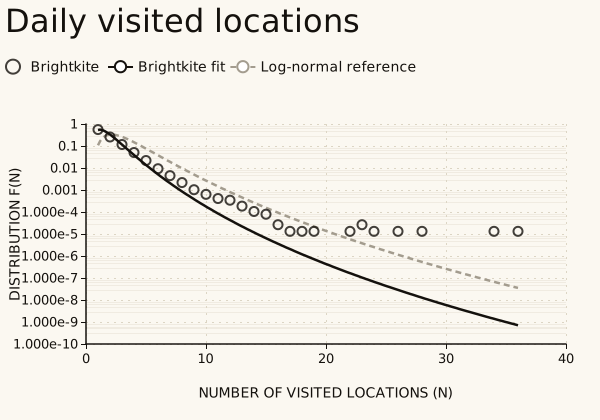
The points are the share of person-days with each number of distinct places (mu = 0.44, sigma = 0.54 for the fit; the dashed curve is a log-normal reference with mu = 1 and sigma = 0.5). Most person-days have one or two places. The fit falls below the points beyond about 15 places, where a few person-days have many check-ins.
Visits, activities and mobility profiles
The remaining charts describe visits to places, so we switch to GPS data. We take six users of GeoLife, detect their stops, cluster the stops into places and label each place home, work or other, exactly as in Visit-based measures.
import fastmob.measures.individual as measures
from fastmob.data import load_geolife

tdf = load_geolife(users=[f"{i:03d}" for i in range(6)], max_trips_per_user=80)
tdf.timezone_conversion(from_timezone="UTC", to_timezone="Asia/Shanghai")
fixes = fastmob.filter(tdf.to_pandas(), max_speed_kmh=200)
staypoints = fastmob.Positionfixes(fixes).generate_staypoints(
    minutes_for_a_stop=20, spatial_radius_km=0.2, no_data_for_minutes=30
)
locations, staypoints = staypoints.generate_user_locations(epsilon_km=0.2)
locations = locations.identify(staypoints)
purposes = locations.to_pandas()[["uid", "location_id", "purpose"]]
visits = (
    staypoints.to_pandas()
    .merge(purposes, on=["uid", "location_id"])
    .rename(columns={"uid": "user_id"})
)

geo_users = sorted(visits["user_id"].unique())
first = visits[visits["user_id"].isin(geo_users[:3])]
second = visits[visits["user_id"].isin(geo_users[3:])]
print(
    len(visits),
    "visits by",
    len(geo_users),
    "users:",
    len(first),
    "by the first three,",
    len(second),
    "by the other three",
)
Visit purposes
visit_purpose_distribution counts visits by purpose; plot_visit_purpose_distribution draws the percentages. plot_visit_purpose_comparison takes a mapping from a name to a distribution and draws them side by side.
from fastmob_vis import (
    plot_visit_purpose_comparison,
    plot_visit_purpose_distribution,
)

distribution = measures.visit_purpose_distribution(visits, activity_col="purpose")
plot_visit_purpose_distribution(distribution)
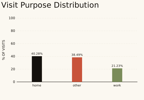
Of the 504 visits, 40% are at a place labelled home (203 visits), 38% at other places (194) and 21% at work (107). The labels come from the rules in Visit-based measures; they are inferred, not observed.
by_group = {
    "first three users": measures.visit_purpose_distribution(
        first, activity_col="purpose"
    ),
    "other three users": measures.visit_purpose_distribution(
        second, activity_col="purpose"
    ),
}
print(
    pd.DataFrame(
        {
            name: table.set_index("activity")["percentage"]
            for name, table in by_group.items()
        }
    ).round(1)
)
plot_visit_purpose_comparison(by_group)
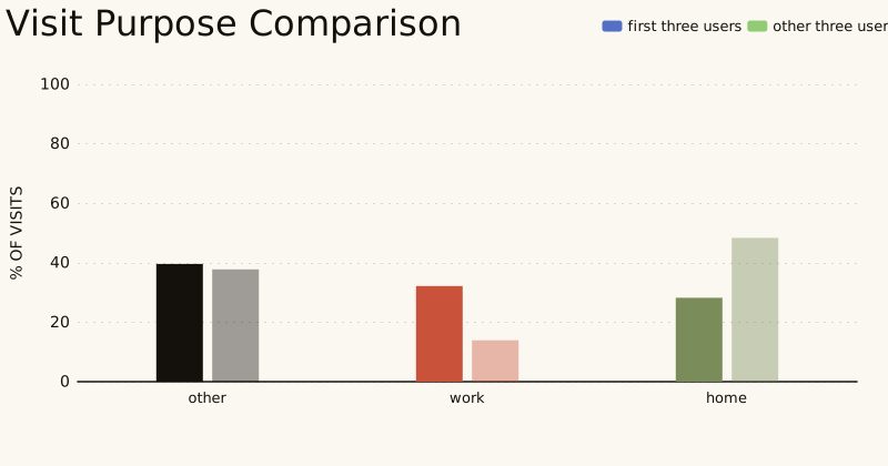
The first three users spend 28% of their visits at home, 40% at other places and 32% at work. The other three spend 48% at home, 38% elsewhere and only 14% at work. With three people in each group and 202 and 302 visits this describes six people, not two populations.
Moving between activities
activity_transition_matrix gives the percentage of visits to each activity that are followed by each activity. plot_activity_transition_matrix draws it as a heatmap (rows are the activity left, columns the activity entered) and plot_activity_transition_difference draws the second matrix minus the first, in percentage points.
from fastmob_vis import (
    plot_activity_transition_difference,
    plot_activity_transition_matrix,
)

transition_kwargs = {
    "activity_col": "purpose",
    "user_id_col": "user_id",
    "timestamp_col": "started_at",
}
transitions = measures.activity_transition_matrix(visits, **transition_kwargs)
plot_activity_transition_matrix(transitions)
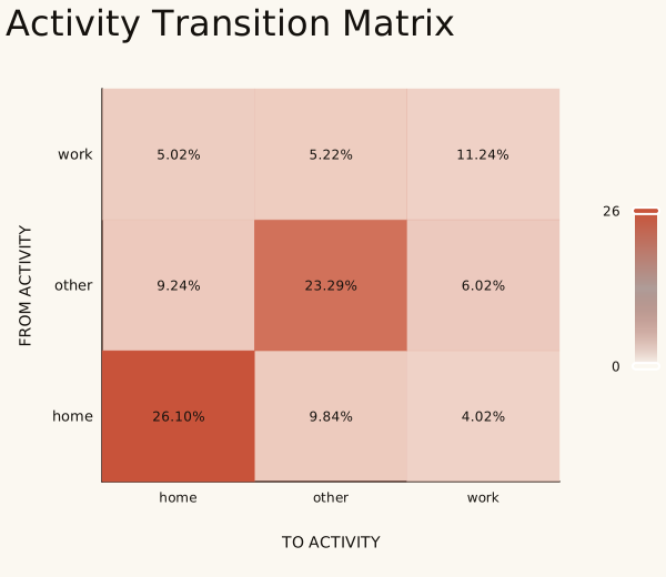
Each cell is the share of all pairs of consecutive visits that go from the row activity to the column activity, so the nine cells add up to 100%. The largest cells are on the diagonal: consecutive visits of the same type, home to home (26%) and other to other (23%).
plot_activity_transition_difference(
    measures.activity_transition_matrix(first, **transition_kwargs),
    measures.activity_transition_matrix(second, **transition_kwargs),
    labels=("first three", "other three"),
)
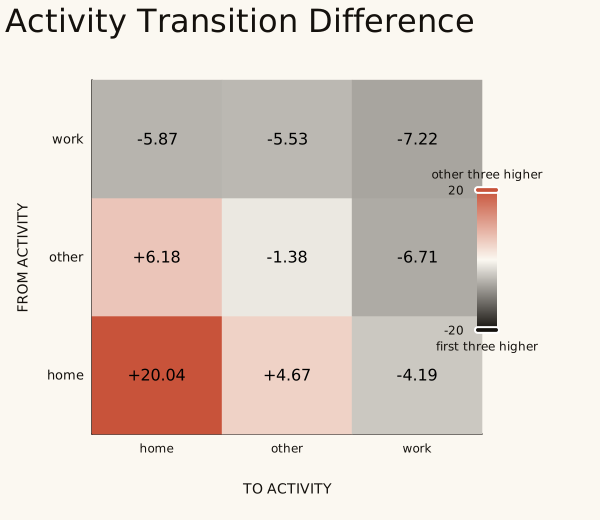
A red cell is a move that the other three users make more often than the first three, and a dark cell one that they make less often (second minus first, in percentage points). The biggest difference is home to home, 20 points higher for the other three (34% against 14%), which matches their larger share of visits at home. Work to work is 7 points lower.
Activities through the day
daily_activity_distribution returns, for each activity, the percentage of visits under way in each 10-minute bin of the day, together with the activity names and the number of bins. plot_daily_activity_distribution draws that tuple as a heatmap, and plot_daily_activity_difference draws the difference between two of them.
from fastmob_vis import (
    plot_daily_activity_difference,
    plot_daily_activity_distribution,
)

daily_kwargs = {
    "activity_col": "purpose",
    "start_time_col": "started_at",
    "end_time_col": "finished_at",
    "bin_size_minutes": 10,
}
daily = measures.daily_activity_distribution(visits, **daily_kwargs)
plot_daily_activity_distribution(daily)
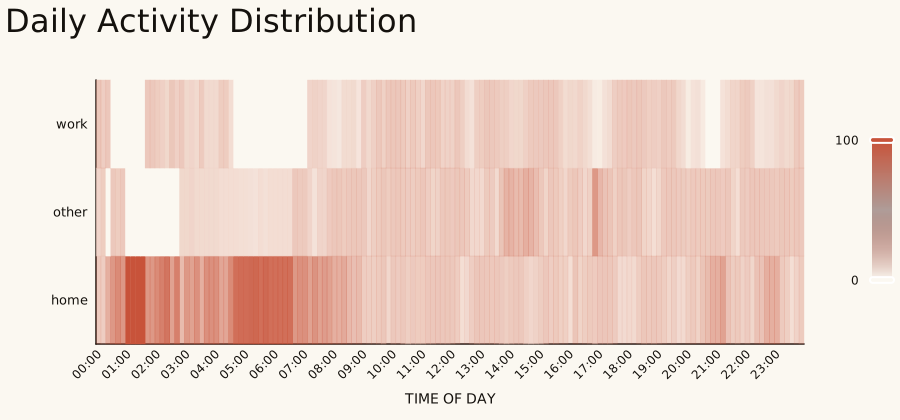
Each column is a 10-minute bin of the day in Beijing time (the time zone we converted to), and each row is an activity. A darker cell means that more of the visits under way in that bin are of that type. Home is the darkest row in the early hours, as expected.
plot_daily_activity_difference(
    measures.daily_activity_distribution(first, **daily_kwargs),
    measures.daily_activity_distribution(second, **daily_kwargs),
    labels=("first three", "other three"),
)
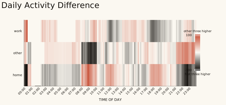
The same difference as before, now through the day: red where the other three users spend more of that bin on the activity, dark where they spend less. With three users per group single bins are noisy, so look for broad bands rather than single cells.
Time spent and time between visits
The same ECDF helpers draw durations. The dwell time of a visit is how long the person stayed; the time between visits is the gap from the end of one visit to the start of the next for the same person, which bounds the duration of the trip in between from above.
from fastmob_vis import plot_dwell_time_ecdf, plot_trip_duration_ecdf

minutes = lambda delta: delta.dt.total_seconds() / 60
ordered = visits.sort_values(["user_id", "started_at"])
gap = ordered["started_at"] - ordered.groupby("user_id")["finished_at"].shift()
dwell = minutes(visits["finished_at"] - visits["started_at"])
in_first = visits["user_id"].isin(geo_users[:3])

plot_dwell_time_ecdf(
    dwell[in_first], dwell[~in_first], labels=("first three", "other three")
)
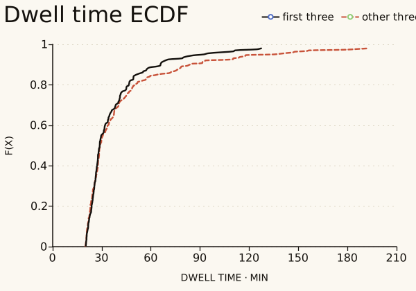
No visit is shorter than 20 minutes, because 20 minutes is the minimum duration we asked for when detecting stops. The median dwell time is 29 minutes in both groups and nine in ten visits last under 78 minutes. The other three users have the longer tail, up to about 190 minutes.
gap_minutes = minutes(gap).dropna()
first_gap = gap_minutes[ordered.loc[gap_minutes.index, "user_id"].isin(geo_users[:3])]
second_gap = gap_minutes.drop(first_gap.index)
plot_trip_duration_ecdf(
    first_gap,
    second_gap,
    labels=("first three", "other three"),
    title="Time between visits",
    x_label="time between visits",
)
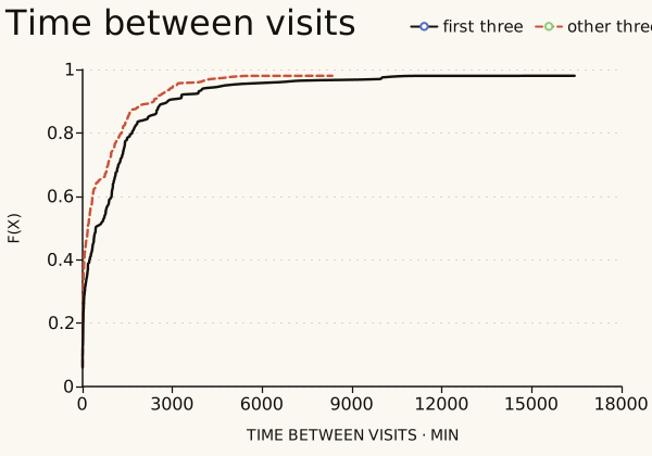
The helper is made for trip durations, but we have visits, not trips, so we gave it the time between the end of one visit and the start of the next (title and x_label change the labels). Half of these gaps are under 266 minutes and 36% under an hour, but nine in ten are under 2,520 minutes (42 hours) and the longest is about 117 days. These gaps include nights and weeks without recording, so they are not trip durations; for those, use the trips of the trajectory hierarchy.
Mobility profiles
compute_profiles gives each person a profile (scouters, regulars or routiners) from how often they return to their places and how often they explore new ones. plot_mobility_profiles plots intermittency against the degree of return with a colour for each profile, and plot_profile_metrics draws a box plot of each metric by profile. Our column is called profile, so we pass profile_col.
from fastmob_vis import plot_mobility_profiles, plot_profile_metrics

profiles = measures.compute_profiles(
    visits,
    user_id_col="user_id",
    location_id_col="location_id",
    start_col="started_at",
    end_col="finished_at",
    purpose_col="purpose",
    n_clusters=3,
    random_state=0,
)
print(profiles["profile"].value_counts().to_dict())
plot_mobility_profiles(profiles, profile_col="profile")
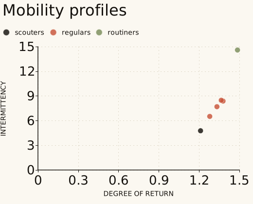
Each point is one person: one scouter, four regulars and one routiner. With six people the groups only illustrate the chart, and they come from clustering these same six, so they say nothing about how many people of each type exist.
plot_profile_metrics(
    {"GeoLife": profiles},
    profile_col="profile",
    profile_order=("scouters", "regulars", "routiners"),
)
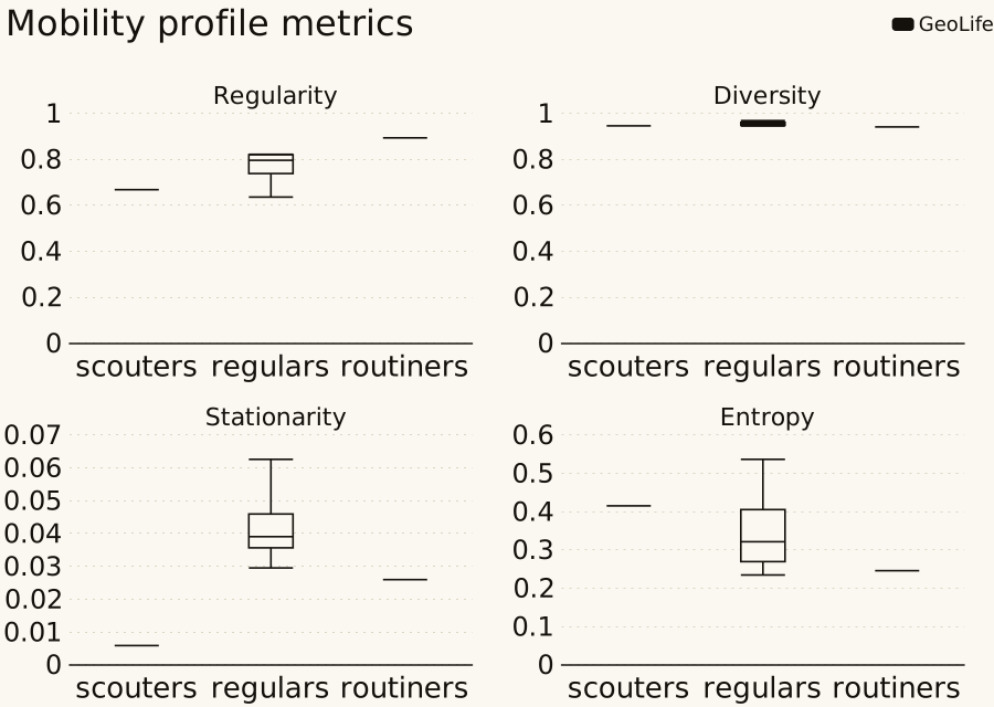
One panel per metric, with the profiles along the horizontal axis. With one scouter and one routiner, their boxes collapse to a line: only the four regulars have a spread. With more people each box shows the variation within a profile.
Daily motifs
A daily motif is the pattern of places a person visits in a day, with the place order and repeats encoded in one integer. plot_motif_literature_comparison compares the share of each motif with the 17 most common motifs of Schneider et al. (2013), which the library ships; the remaining motifs are summed in an other bar.
from fastmob_vis import plot_motif_literature_comparison

daily_motifs = staypoints.generate_daily_motifs(locations)
motifs = measures.motif_distribution(daily_motifs)
plot_motif_literature_comparison(
    reference_distribution=motifs, labels=("GeoLife", "Simulation")
)
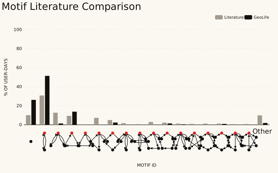
The light bars are the shares of the 17 most common daily motifs in the literature and the dark bars are the shares in these data (the motifs outside the 17 are summed in the last bar). Of the 210 person-days here, 51% have the second motif (a day spent at two places) against 31% in the literature, which says as much about this small GeoLife sample as about behaviour.
Maps, which are interactive only
map draws the polygons of a GeoJSON FeatureCollection, and plot_stvd_comparison draws a spatio-temporal visitation difference over a map from OpenStreetMap, with the zoom level choosing between H3 resolutions. Both need JavaScript and, for the second, an internet connection for the tiles, so they are not drawn on this page and cannot be exported as SVG. This is the shape of the input, with three invented zones; in a notebook the last line draws the map.
from fastmob_vis import plot_stvd_comparison


def zone(name, lng, lat, volume_diff_pct, peak_shift_hours, size=0.01):
    ring = [
        [lng, lat],
        [lng + size, lat],
        [lng + size, lat + size],
        [lng, lat + size],
        [lng, lat],
    ]
    return {
        "type": "Feature",
        "geometry": {"type": "Polygon", "coordinates": [ring]},
        "properties": {
            "area": name,
            "volume_diff_pct": volume_diff_pct,
            "peak_shift_hours": peak_shift_hours,
        },
    }


layers = {
    8: {
        "type": "FeatureCollection",
        "features": [
            zone("north", 116.30, 39.99, 9.0, 1.5),
            zone("centre", 116.31, 39.98, -4.0, 0.5),
            zone("south", 116.30, 39.97, 1.0, 6.0),
        ],
    }
}
comparison = plot_stvd_comparison(layers, volume_threshold=3.0)
zones = vis.map(layers[8], title="Three invented zones")
print(
    zones.kind,
    "chart;",
    len(layers[8]["features"]),
    "zones;",
    type(comparison).__name__,
)
The three properties are the volume difference between the two data sets in percent (positive when the second has more visits), the shift of the daily peak in hours (0 to 12) and an area name for the tooltip. volume_threshold (percent) separates the colour bins.
Save and embed charts
A Chart can be exported as a standalone page, as the ECharts option in JSON (what a web application passes to ECharts) or as a plain SVG. The SVG is a simple drawing without axis labels or a legend, enough for a thumbnail; use the page for a chart that you share. To put several charts on one page, write the JavaScript libraries once with get_resource_bundle and make each chart with bundle_libs=False.
chart = vis.ecdf(jumps_a, value_col="jump_lengths", x_unit="km")
saved = {
    "html": chart.to_html("jump-lengths.html"),
    "json": chart.to_json("jump-lengths.json"),
    "svg": chart.to_svg("jump-lengths.svg"),
}
pd.Series(
    {kind: f"{path.stat().st_size / 1024:,.0f} KB" for kind, path in saved.items()},
    name="size",
)
head = vis.get_resource_bundle()
light = vis.ecdf(jumps_a, value_col="jump_lengths", bundle_libs=False)
figure = light.render()
print(f"The libraries are {len(head) / 1024:,.0f} KB, written once by the bundle.")
print(
    f"{type(figure).__name__}: the lower-level figure, with {len(figure.to_dict())} option keys"
)
The libraries are 1,009 KB, written once by the bundle.
EChartsFigure: the lower-level figure, with 11 option keys
The standalone page is about a megabyte because it embeds the ECharts library; the JSON and the SVG are small. The SVG written by to_svg is a plain drawing without axis labels or a legend. For a chart to share, save the page or draw the JSON with ECharts, and with bundle_libs=False write the libraries once for a page of charts.
Interpretation and limits
- A chart draws what it is given. The ECDF of jump lengths of a few hundred people says nothing about a population, and the two samples here were split arbitrarily, so a difference between them is only an illustration.
- The generic charts need one row per mark.
bar,boxplotandheatmapdo not aggregate: they use the first row for a repeated category and draw 0 for a missing one, so aggregate first. - The ECDF curves stop at the 98th percentile. Raise
cdf_cutoffto see the tail. - Pictures made from a chart have no tooltips, and maps cannot be exported as pictures.
plot_motif_literature_comparisoncompares shares of motifs, which depend on how stops and places were found; they are not directly comparable between data sets.
Next steps
- Compare simulated and observed results: Generate mobility.
- Understand the fitted laws behind the three law charts: Compare to mobility laws.
- See every chart option and function: Visualization reference.
Related API
ecdf ·
bar ·
boxplot ·
scatter ·
heatmap ·
map ·
Chart ·
get_resource_bundle ·
plot_jump_lengths_ecdf ·
plot_radius_of_gyration_ecdf ·
plot_visits_frequency_ecdf ·
plot_trip_duration_ecdf ·
plot_dwell_time_ecdf ·
plot_visit_purpose_distribution ·
plot_visit_purpose_comparison ·
plot_activity_transition_matrix ·
plot_activity_transition_difference ·
plot_daily_activity_distribution ·
plot_daily_activity_difference ·
plot_mobility_profiles ·
plot_profile_metrics ·
plot_motif_literature_comparison ·
plot_truncated_powerlaw_fits ·
plot_lognormal_fits ·
plot_distance_frequency_law ·
plot_stvd_comparison