

Routine, predictability and mobility profiles
Question. How regular, diverse and predictable is each person's routine, and what kinds of people (routine followers, explorers) are in my sample?
You will get a visit table (one row per stop, with a place and a purpose), and per-person regularity, diversity, entropy, predictability, return and exploration measures, the mix of visit purposes, how people move between purposes, how activities are spread over the day, and a clustering of people into mobility profiles.
Prerequisites. Build the trajectory hierarchy: stops, trips and tours: this notebook starts from the stops and places it produces.
Data. GeoLife: the first 80 trips of users 000 to 005 (about 630,000 fixes, roughly 25 MB read from the 313 MB archive) with fastmob.data.load_geolife. Timestamps are converted from UTC to Beijing time first, because home and work are defined by the hour of the day. The notebook stops if the download fails.
From fixes to a visit table
Visit-based measures need one row per visit: who, where (a place id) and, optionally, when and for what purpose. We build it from GeoLife in four steps: convert to local time, detect stops, group stops into per-person places, and label the places home, work or other.
import fastmob
from fastmob.data import load_geolife

tdf = load_geolife(users=[f"{i:03d}" for i in range(6)], max_trips_per_user=80)

tdf.timezone_conversion(from_timezone="UTC", to_timezone="Asia/Shanghai")
fixes = fastmob.filter(tdf.to_pandas(), max_speed_kmh=200)
staypoints = fastmob.Positionfixes(fixes).generate_staypoints(
    minutes_for_a_stop=20, spatial_radius_km=0.2, no_data_for_minutes=30
)
locations, staypoints = staypoints.generate_user_locations(epsilon_km=0.2)
locations = locations.identify(staypoints)
purposes = locations.to_pandas()[["uid", "location_id", "purpose"]]
visits = (
    staypoints.to_pandas()
    .merge(purposes, on=["uid", "location_id"])
    .rename(columns={"uid": "user_id"})
)

print(
    len(fixes),
    "fixes ->",
    len(visits),
    "visits by",
    visits["user_id"].nunique(),
    "users",
)
visits.groupby("user_id").size().rename("visits").to_frame().T
| user_id | 000 | 001 | 002 | 003 | 004 | 005 |
|---|---|---|---|---|---|---|
| visits | 51 | 52 | 99 | 117 | 83 | 102 |
The 630,771 fixes became 504 visits by six users, between 51 and 117 per user. Each visit has the user, the stop times, the place id and its purpose.
How far did they travel in total?
distance_straight_line is the total length of a person's trajectory, in kilometres, adding up the straight-line distances between consecutive fixes. It uses the fixes, not the visits.
| uid | distance_straight_line | |
|---|---|---|
| 0 | 000 | 1641.663542 |
| 1 | 001 | 1013.679754 |
| 2 | 002 | 1781.410094 |
| 3 | 003 | 2039.564706 |
| 4 | 004 | 1192.089474 |
| 5 | 005 | 6052.488847 |
Distances add up over all recorded days, so they depend on how much each person was recorded: user 005's 6,052 km against about 1,000 to 2,000 km for most others says as much about recording volume as about travel. Divide by the number of recorded days before comparing people.
How regular, diverse and predictable?
regularity is 1 minus the number of distinct places divided by the number of visits, so it is high when a person keeps returning to the same few places. diversity is the share of distinct sub-sequences in the person's sequence of places (higher means a more varied sequence). trajectory_entropy is a normalised (0 to 1) entropy of that sequence. real_entropy and trajectory_predictability use the order of visits: the entropy is in bits, and the predictability is the highest share of next places an ideal predictor could get right (Fano's bound).
import fastmob.measures.individual as measures

regularity = measures.regularity(
    visits,
    user_id_col="user_id",
    location_id_col="location_id",
    location_type_col="purpose",
)
diversity = measures.diversity(
    visits, user_id_col="user_id", location_id_col="location_id"
)
entropy = measures.trajectory_entropy(
    visits,
    user_id_col="user_id",
    location_id_col="location_id",
    timestamp_col="started_at",
)
real = measures.real_entropy(
    visits, uid_col="user_id", location_id_col="location_id", datetime_col="started_at"
)
predictability = measures.trajectory_predictability(
    visits,
    user_id_col="user_id",
    location_id_col="location_id",
    timestamp_col="started_at",
)

summary = (
    regularity.merge(diversity)
    .merge(entropy)
    .merge(predictability, on="user_id")
    .rename(columns={"real_entropy": "real_entropy_bits"})
)
print(real.round(2).to_string())
summary.round(2)
| user_id | regularity | diversity | entropy | real_entropy_bits | predictability | n_unique_locations | n_steps | |
|---|---|---|---|---|---|---|---|---|
| 0 | 000 | 0.67 | 0.94 | 0.41 | 2.35 | 0.65 | 17 | 51 |
| 1 | 001 | 0.63 | 0.97 | 0.54 | 3.06 | 0.51 | 19 | 52 |
| 2 | 002 | 0.82 | 0.95 | 0.28 | 1.86 | 0.75 | 18 | 99 |
| 3 | 003 | 0.82 | 0.94 | 0.23 | 1.61 | 0.80 | 21 | 117 |
| 4 | 004 | 0.77 | 0.96 | 0.36 | 2.30 | 0.67 | 19 | 83 |
| 5 | 005 | 0.89 | 0.94 | 0.25 | 1.64 | 0.75 | 11 | 102 |
The first table printed above is real_entropy on its own, from 1.61 bits (user 003) to 3.06 bits (user 001); the same values appear as real_entropy_bits in the summary. User 005 is the most regular: 11 distinct places in 102 visits give a regularity of 0.89, and an ideal predictor could guess their next place 75% of the time. User 001 is the least: 19 places in 52 visits give 0.63, with a predictability of 0.51. User 003 has the lowest normalised entropy (0.23) and the highest predictability (0.80). Diversity is about 0.95 for everyone, so it does not separate these six people.
Return and exploration
intermittance_and_degree_of_return splits each person's movement into returns to known places and explorations of new ones: intermittency is the typical number of visits between new places, degree of return how often they come back, and mean_return and mean_exploration the average run lengths. exploration_profiling adds a three-way label based on these (routiners, regulars, scouters).
returns = measures.intermittance_and_degree_of_return(
    visits,
    user_id_col="user_id",
    location_id_col="location_id",
    datetime_col="started_at",
)
profiles = measures.exploration_profiling(
    visits,
    user_id_col="user_id",
    location_id_col="location_id",
    datetime_col="started_at",
)

print(returns.round(2).to_string())
profiles.round(2)
  user_id  intermittency  degree_of_return  mean_return  mean_exploration
0     000           4.75              1.21         3.45              1.30
1     001           6.50              1.28         5.00              1.50
2     002           8.36              1.38         7.00              1.36
3     003           8.46              1.36         7.00              1.46
4     004           7.68              1.33         6.18              1.50
5     005          14.57              1.49        13.43              1.14
| user_id | intermittency | degree_of_return | mean_return | mean_exploration | profile | |
|---|---|---|---|---|---|---|
| 0 | 000 | 4.75 | 1.21 | 3.45 | 1.30 | scouters |
| 1 | 001 | 6.50 | 1.28 | 5.00 | 1.50 | scouters |
| 2 | 002 | 8.36 | 1.38 | 7.00 | 1.36 | regulars |
| 3 | 003 | 8.46 | 1.36 | 7.00 | 1.46 | regulars |
| 4 | 004 | 7.68 | 1.33 | 6.18 | 1.50 | regulars |
| 5 | 005 | 14.57 | 1.49 | 13.43 | 1.14 | routiners |
User 005 returns to known places for long runs before exploring a new one (intermittency 14.6, mean return 13.4 visits) and is labelled a routiner; users 000 and 001, who explore after much shorter runs (4.8 and 6.5), are scouters; the others are regulars. The table printed above the profiles is the raw output of intermittance_and_degree_of_return: user 005 has the highest intermittency (14.57) and degree of return (1.49), user 000 the lowest (4.75 and 1.21).
Predict the next place
NextLocationPredictor is a Markov model of order k: it predicts a person's next place from their last k places. fit learns from the visit sequences (ordered by started_at); with backoff=True an unseen context falls back to shorter ones. predict returns the single most likely next place of each person after their last visit, predict_proba the top_k most likely places with their probabilities, and evaluate hides the last n_holdout visits of each person and reports the share of them that the model puts in its top_k guesses.
from fastmob.models import NextLocationPredictor

predictor = NextLocationPredictor(order=1, backoff=True).fit(
    visits, location_col="location_id", uid_col="user_id", started_at_col="started_at"
)
next_place = predictor.predict(top_k=1)
print(next_place.to_string())
next_proba = predictor.predict_proba(top_k=3)
accuracy = {k: predictor.evaluate(top_k=k, n_holdout=10) for k in (1, 3)}

print(
    {k: round(v, 2) for k, v in accuracy.items()},
    "(share of held-out visits predicted in the top k)",
)
baseline = NextLocationPredictor(order=0).fit(
    visits, location_col="location_id", uid_col="user_id", started_at_col="started_at"
)
baseline_accuracy = {k: baseline.evaluate(top_k=k, n_holdout=10) for k in (1, 3)}
print(
    {k: round(v, 2) for k, v in baseline_accuracy.items()},
    "(order-0 baseline: always the most frequent place)",
)
next_proba.head(6)
  user_id  location_id
0     000            1
1     001            0
2     002            0
3     003            0
4     004            0
5     005            1
{1: 0.42, 3: 0.63} (share of held-out visits predicted in the top k)
{1: 0.45, 3: 0.68} (order-0 baseline: always the most frequent place)
| user_id | rank | location_id | probability | |
|---|---|---|---|---|
| 0 | 000 | 1 | 1 | 1.000000 |
| 1 | 001 | 1 | 0 | 0.250000 |
| 2 | 001 | 2 | 1 | 0.153846 |
| 3 | 001 | 3 | 2 | 0.076923 |
| 4 | 002 | 1 | 0 | 0.608696 |
| 5 | 002 | 2 | 1 | 0.217391 |
Holding out the last ten visits of each person, the model finds the next place in its first guess for 42% of them and within its three best guesses for 63%. For user 000 the single most likely next place has probability 1.0 only because that place always followed the current one in their short history (51 visits); for user 001 the three best guesses have probabilities 0.25, 0.15 and 0.08. Consecutive visits to the same place are common in this table, which makes a first-order model look better than it would on a table with one row per change of place, so compare with the order-0 baseline (NextLocationPredictor(order=0), always the most frequent place). The baseline does slightly better here (45% in its first guess and 68% within three), so the first-order model adds nothing on this small sample: do not read 42% as predictive skill.
One table of profiles
compute_profiles combines these measures with regularity, diversity, entropy and stationarity (the time a person spends at their places divided by the time between their first and last stay), and clusters the people on their standardised intermittency and degree of return with k-means (up to three clusters get the names routiners, regulars and scouters).
combined = measures.compute_profiles(
    visits,
    user_id_col="user_id",
    location_id_col="location_id",
    start_col="started_at",
    end_col="finished_at",
    purpose_col="purpose",
    n_clusters=3,
    random_state=0,
)
combined.round(2)
| user_id | intermittency | degree_of_return | regularity | diversity | entropy | stationarity | profile | |
|---|---|---|---|---|---|---|---|---|
| 0 | 000 | 4.75 | 1.21 | 0.67 | 0.94 | 0.41 | 0.00579 | scouters |
| 1 | 001 | 6.50 | 1.28 | 0.63 | 0.97 | 0.54 | 0.029443 | regulars |
| 2 | 002 | 8.36 | 1.38 | 0.82 | 0.95 | 0.28 | 0.03762 | regulars |
| 3 | 003 | 8.46 | 1.36 | 0.82 | 0.94 | 0.23 | 0.062528 | regulars |
| 4 | 004 | 7.68 | 1.33 | 0.77 | 0.96 | 0.36 | 0.040323 | regulars |
| 5 | 005 | 14.57 | 1.49 | 0.89 | 0.94 | 0.25 | 0.025876 | routiners |
The clusters agree with the previous table except for user 001, who is a scout in exploration_profiling and a regular here. With six people the cluster boundaries are unstable, and the two functions fit their clusters separately, so profile names should not be compared across runs or samples.
What are people doing?
visit_purpose_distribution counts the visits of each purpose. activity_transition_matrix gives the percentage of consecutive visits that go from one purpose (rows) to another (columns). daily_activity_distribution returns, for each 10-minute bin of the day, the percentage of the observed activity that falls in each purpose.
distribution = measures.visit_purpose_distribution(visits, activity_col="purpose")
transitions = measures.activity_transition_matrix(
    visits, activity_col="purpose", user_id_col="user_id", timestamp_col="started_at"
)
matrix, activities, bins = measures.daily_activity_distribution(
    visits,
    activity_col="purpose",
    start_time_col="started_at",
    end_time_col="finished_at",
    bin_size_minutes=10,
)

print(distribution.round(1).to_string(index=False))
transitions.round(1)
| activity | home | other | work | |
|---|---|---|---|---|
| 0 | home | 26.1 | 9.8 | 4.0 |
| 1 | other | 9.2 | 23.3 | 6.0 |
| 2 | work | 5.0 | 5.2 | 11.2 |
Home takes 40% of the visits, other places 38.5% and work 21%. In the transition matrix (the nine cells sum to 100% of consecutive visit pairs, rows are the origin purpose and columns the destination), most transitions stay within the same purpose: home to home 26.1%, other to other 23.3%, work to work 11.2%. Consecutive stops at the same purpose are common because a visit to one place can be split into several stops.
import matplotlib.pyplot as plt

fig, ax = plt.subplots(figsize=(7, 3))
hours = [i * 10 / 60 for i in range(matrix.shape[1])]
for row, label in zip(matrix, activities):
    ax.plot(hours, row, label=label)
ax.set_xlabel("hour of the day (Beijing time)")
ax.set_ylabel("% of visits at that time")
ax.set_xlim(0, 24)
ax.set_xticks(range(0, 25, 3))
ax.legend()
plt.show()
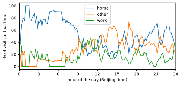
Each curve shows, for each 10-minute bin of the Beijing day, the share of the observed activity that falls in each purpose. With six people the curves are jagged, and the shares in a bin always add up to about 100%.
Interpretation and limits
- Six people and 504 visits are far too few for population statements. The point is how to run and read the measures.
- Purposes are
home,workorotherfrom a dwell-time rule on stay times (night and weekday daytime hours, in Beijing time here). They are guesses and driveregularity, the purpose distribution and the transition matrix. - Entropy and predictability depend on how places are defined: finer places make people look less predictable. Report the clustering radius.
- Profile names come from the clustering of these six people only; with other users the same person could change cluster.
Next steps
- Day-by-day patterns of the same visits: Find daily mobility motifs.
- Population-level summaries: Population measures.
Related API
NextLocationPredictor ·
distance_straight_line ·
regularity ·
diversity ·
trajectory_entropy ·
real_entropy ·
trajectory_predictability ·
intermittance_and_degree_of_return ·
exploration_profiling ·
compute_profiles ·
visit_purpose_distribution ·
activity_transition_matrix ·
daily_activity_distribution