

Measure individual mobility
Question. How far, how often and how predictably does each person move, and which places matter to them?
You will get per-person values for range, number of places, visit counts, place-visit entropy, inferred home and work, and ranked place lists, plus population-level distributions of the main ones.
Prerequisites. The trajectory table and the idea of a measure per person (Start with a trajectory).
Data. Brightkite, location check-ins from a location-based social network (Stanford SNAP, 2008 to 2010). The full file is about 60 MB; fastmob.data.load_brightkite streams it and stops after 300,000 rows, about 4 MB. Users with fewer than 100 check-ins in that window are dropped, which leaves about 306 users and 283,500 check-ins (after also removing placeholder coordinates, see below). Check-ins are voluntary and sparse, so they describe where people chose to check in rather than all their movement.
Load the data
load_brightkite downloads the first rows of the file and returns a trajectory table with uid, datetime, lat and lng. We drop users with fewer than 100 check-ins, which are too few for stable per-person measures.
import fastmob
from fastmob.data import load_brightkite

checkins = load_brightkite(max_rows=300_000).to_pandas()

null_island = ((checkins["lat"] == 0) & (checkins["lng"] == 0)) | (
    checkins["lat"].abs() >= 90
)
print(
    f"dropping {null_island.sum()} check-ins at latitude 0, longitude 0 (a placeholder for 'unknown') or with an impossible latitude"
)
checkins = checkins[~null_island]
counts = checkins.groupby("uid").size()
checkins = checkins[checkins["uid"].isin(counts[counts >= 100].index)].reset_index(
    drop=True
)
print(len(checkins), "check-ins from", checkins["uid"].nunique(), "users")
checkins.head()
dropping 8327 check-ins at latitude 0, longitude 0 (a placeholder for 'unknown') or with an impossible latitude
283543 check-ins from 306 users
| uid | datetime | lat | lng | |
|---|---|---|---|---|
| 0 | 0 | 2010-10-17 01:48:53 | 39.747652 | -104.992510 |
| 1 | 0 | 2010-10-16 06:02:04 | 39.891383 | -105.070814 |
| 2 | 0 | 2010-10-16 03:48:54 | 39.891077 | -105.068532 |
| 3 | 0 | 2010-10-14 18:25:51 | 39.750469 | -104.999073 |
| 4 | 0 | 2010-10-14 00:21:47 | 39.752713 | -104.996337 |
Units and assumptions
- Distances are in kilometres, waiting times in seconds.
- Times are UTC. Measures that depend on the hour of day (home, work) treat hours as UTC, so a user in San Francisco has "night" shifted by eight hours. For a real study convert
datetimeto local time first. - Users are identified by
uid; without it all rows are treated as one person. - Check the data first. Brightkite contains check-ins at exactly latitude 0, longitude 0 (a point in the Atlantic Ocean), which are placeholders for an unknown location, and a few rows whose latitude is 90 degrees or beyond, which is impossible (the coordinates are swapped or invalid). Left in, they would make some users appear to travel thousands of kilometres. The cell above removes them and reports how many there were.
How far and how widely: radius of gyration, maximum distance, jump lengths
radius_of_gyration is the typical distance of a user's check-ins from their centre of mass; k_radius_of_gyration computes it from only the user's k most visited places. maximum_distance is the largest distance between two consecutive check-ins of a user, that is, their longest single jump (not the span between their two most distant places).
rg = fastmob.radius_of_gyration(checkins)
krg = fastmob.k_radius_of_gyration(checkins, k=2)
max_dist = fastmob.maximum_distance(checkins)

ranges = rg.merge(krg, on="uid").merge(max_dist, on="uid")
ranges.describe().round(1)
| radius_of_gyration | k_radius_of_gyration | maximum_distance | |
|---|---|---|---|
| count | 306.0 | 306.0 | 306.0 |
| mean | 1001.4 | 155.4 | 5767.7 |
| std | 1250.1 | 897.3 | 4579.4 |
| min | 0.0 | 0.0 | 0.0 |
| 25% | 294.6 | 1.0 | 1953.5 |
| 50% | 699.1 | 4.2 | 4152.6 |
| 75% | 1269.3 | 11.7 | 9132.1 |
| max | 13434.5 | 13840.8 | 16954.2 |
The median user has a radius of gyration of about 700 km and a maximum distance of about 4,000 km: Brightkite users are spread across the world and many travel between cities or continents, so the distribution is wide and heavy-tailed. k_radius_of_gyration with k=2 has a median of only about 4 km, which means that for a typical user the two most visited places lie within a few kilometres of each other; the large overall radius comes from the other, less visited places.
import matplotlib.pyplot as plt
import numpy as np

fig, ax = plt.subplots(figsize=(6, 3.5))
ax.hist(np.log10(rg["radius_of_gyration"].clip(lower=0.01)), bins=40, color="#a98600")
ax.set_xlabel("log10 radius of gyration (km)")
ax.set_ylabel("users")
ax.set_title("Brightkite users: how widely they range")
plt.show()
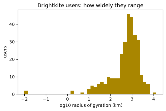
Radii span several orders of magnitude, from under a kilometre to over ten thousand, so the histogram uses a log axis. Radii below 0.01 km (a user who always checks in at one place) are clipped to 0.01 km and fall in the left-most bar. For such data report medians or quantiles rather than means, which the long tail dominates.
jump_lengths and waiting_times return one list of values per user; merge=True returns them as one flat array for pooled distributions.
jumps = fastmob.jump_lengths(checkins, merge=True)
waits = fastmob.waiting_times(checkins, merge=True)

print(
    f"{len(jumps):,} jumps, median {np.median(jumps):.2f} km, 95th percentile {np.percentile(jumps, 95):.0f} km"
)
print(f"{len(waits):,} waits, median {np.median(waits) / 3600:.1f} h")
The median jump is 0 km because people often check in repeatedly at the same venue, while the 95th percentile is about 58 km, the same heavy tail seen above. Check-in waits are measured in hours (median about 2) because people check in occasionally.
How many places: locations, visits and entropy
A location here is a distinct coordinate pair. number_of_locations counts them, number_of_visits counts all check-ins. uncorrelated_entropy measures how evenly check-ins are spread over places (0 means one place; higher means more places visited more evenly), and random_entropy is the entropy if every place were visited equally often, which is just log2 of the number of places.
places = fastmob.number_of_locations(checkins).merge(
    fastmob.number_of_visits(checkins), on="uid"
)
entropy = fastmob.uncorrelated_entropy(checkins).merge(
    fastmob.random_entropy(checkins), on="uid"
)

places.merge(entropy, on="uid").describe().round(2)
| number_of_locations | number_of_visits | uncorrelated_entropy | random_entropy | |
|---|---|---|---|---|
| count | 306.00 | 306.00 | 306.00 | 306.00 |
| mean | 176.39 | 926.61 | 5.04 | 6.79 |
| std | 155.14 | 737.16 | 1.81 | 1.66 |
| min | 1.00 | 105.00 | 0.00 | 0.00 |
| 25% | 65.75 | 284.25 | 3.97 | 6.04 |
| 50% | 125.50 | 637.50 | 5.40 | 6.97 |
| 75% | 235.75 | 1669.00 | 6.39 | 7.88 |
| max | 771.00 | 2100.00 | 8.80 | 9.59 |
The average user has about 176 distinct places for about 927 visits, and the uncorrelated entropy (about 5.0 bits) sits below the random entropy (about 6.8 bits): visits concentrate on a few favourite places instead of spreading evenly. The gap between the two columns is a simple measure of how routine someone's behaviour is.
Which places matter: frequency and recency ranks
location_frequency returns every place of every user with the share of visits it receives; frequency_rank orders them by visits and recency_rank by how recently they were last visited. They return one row per user and place.
top = fastmob.frequency_rank(checkins)
freq = fastmob.location_frequency(checkins)
recent = fastmob.recency_rank(checkins)

first_user = top["uid"].iloc[0]
print("user", first_user, "- most visited places and their share of visits")
top[top["uid"] == first_user].merge(freq, on=["uid", "lat", "lng"]).head(5)
| uid | lat | lng | frequency_rank | location_frequency | |
|---|---|---|---|---|---|
| 0 | 0 | 39.762146 | -104.982480 | 1 | 0.102638 |
| 1 | 0 | 39.891077 | -105.068532 | 2 | 0.065707 |
| 2 | 0 | 39.739154 | -104.984703 | 3 | 0.060432 |
| 3 | 0 | 39.891586 | -105.068463 | 4 | 0.034532 |
| 4 | 0 | 39.827022 | -105.143191 | 5 | 0.025420 |
This user's most visited place receives about 10% of their visits, followed by about 7% and 6%. recency_rank answers a different question: which place was visited last, independent of how often. Here are the same user's most recently visited places.
| uid | lat | lng | recency_rank | |
|---|---|---|---|---|
| 0 | 0 | 39.747652 | -104.992510 | 1 |
| 1 | 0 | 39.891383 | -105.070814 | 2 |
| 2 | 0 | 39.891077 | -105.068532 | 3 |
| 3 | 0 | 39.750469 | -104.999073 | 4 |
| 4 | 0 | 39.752713 | -104.996337 | 5 |
Rank 1 is the place of the user's latest check-in, rank 2 the next most recently visited different place, and so on. The most visited place from the previous table is not among the five most recent: a favourite place can be stale, which is why the two ranks answer different questions.
Home and work
home_location is the place a user visits most between start_night and end_night hours (default 22 to 7); if a user has no check-ins in that window it falls back to their most visited place overall. work_location is the most visited place between 8 and 18 on weekdays (Monday to Friday). max_distance_from_home is the farthest check-in from the inferred home. Remember that the hours, and so the weekdays, are UTC.
homes = fastmob.home_location(checkins)
works = fastmob.work_location(checkins)
away = fastmob.max_distance_from_home(checkins)

hours = checkins["datetime"].dt.hour
night_users = checkins.loc[(hours >= 22) | (hours < 7), "uid"].nunique()
print(
    len(homes),
    "users with an inferred home, of which",
    night_users,
    "have any check-in between 22:00 and 07:00 UTC;",
    len(works),
    "with a work location",
)
homes.merge(away, on="uid").head()
306 users with an inferred home, of which 306 have any check-in between 22:00 and 07:00 UTC; 305 with a work location
| uid | lat | lng | max_distance_from_home | |
|---|---|---|---|---|
| 0 | 0 | 39.891077 | -105.068532 | 8107.017192 |
| 1 | 1 | 37.630490 | -122.411084 | 309.111589 |
| 2 | 2 | 39.739154 | -104.984703 | 8016.409740 |
| 3 | 3 | 37.748170 | -122.459192 | 4343.488499 |
| 4 | 4 | 60.180171 | 24.949728 | 15512.810134 |
Every user has at least one check-in in the UTC night window, so the fallback to the most visited place was not needed here. But the window is UTC, not each user's local night: for a San Francisco user, 22:00 to 07:00 UTC is 14:00 to 23:00 local time, so their inferred "home" mostly reflects afternoon and evening check-ins. Convert datetime to local time before inferring home or work. One of the 306 users has no check-in on a weekday between 08:00 and 18:00 UTC, so work_location returns 305 rows. Either way, a home inferred from social check-ins is a guess about where someone is at night, not a verified address.
A user's mobility network
individual_mobility_network turns a user's check-ins into a directed network whose nodes are places and whose edges count the trips between consecutive places.
network = fastmob.individual_mobility_network(checkins)

network.groupby("uid")["n_trips"].agg(edges="size", trips="sum").describe().round(1)
| edges | trips | |
|---|---|---|
| count | 304.0 | 304.0 |
| mean | 322.2 | 438.7 |
| std | 302.4 | 409.0 |
| min | 2.0 | 2.0 |
| 25% | 107.8 | 134.0 |
| 50% | 215.5 | 269.0 |
| 75% | 443.5 | 627.8 |
| max | 1663.0 | 1999.0 |
The summary covers 304 of the 306 users: two never move between two different places, so they have no edge. The median user has about 216 distinct place-to-place connections for about 269 trips, so most connections are travelled only once or twice: a few routine links plus many one-off trips.
Interpretation and limits
- The numbers describe check-in behaviour. A person's "home" here is the place where they check in at night (or, failing that, where they check in most), which may not be where they live.
- Placeholder (0, 0) coordinates and impossible latitudes were removed; other wrong coordinates may remain.
- Only 300,000 of 4.7 million rows were read, in the file's own order. The first users are not a random sample.
- Distances are straight lines between check-ins; entropies treat each exact coordinate as a place, so GPS noise would inflate them. Cluster stops into places first (Clean noisy GPS data and find stops).
- Time-of-day measures depend on the UTC assumption above.
Next steps
- Population-level summaries, such as visits per location: Population measures.
- Fit a model to the jump-length distribution: Compare your data to mobility laws.
Related API
radius_of_gyration ·
k_radius_of_gyration ·
maximum_distance ·
jump_lengths ·
waiting_times ·
number_of_locations ·
number_of_visits ·
uncorrelated_entropy ·
random_entropy ·
frequency_rank ·
location_frequency ·
recency_rank ·
home_location ·
work_location ·
max_distance_from_home ·
individual_mobility_network